Application · Steel & rolling mill process monitoring
Every cut and every jam on a 140 m/s wire line, recorded around the clock.
In a rolling mill, high-speed shears cut glowing wire that is moving at up to 140 m/s. When a cut comes out uneven or the wire jams and stops production, it is over before anyone can see why. HSCAM STREAMER records every event, keeps a week of history, and lines the video up with the mill’s measurement data.
- Wire speed
- up to 140 m/s
- Wire temperature
- ~1,200 °C
- Exposure
- 100 ns – 3 µs
- History kept
- ≥ 1 week
The situation
Nobody sees the fault happen
Steel wire, up to several centimetres thick and around 1,200 °C, runs through the shear at up to 140 m/s. For no apparent reason, some cut surfaces come out uneven. Quite regularly, a wire jam stops production.
The mill wants to understand both. That means recording every single cut or jam, unattended and around the clock, so that when quality control finds a bad surface, the engineers can go back and watch it in slow motion.
The customer’s verdict on the systems already on the market: they were unreliable at saving high data rates continuously, hard to adapt to the mill’s own process, or lacked exact timing.
System diagram
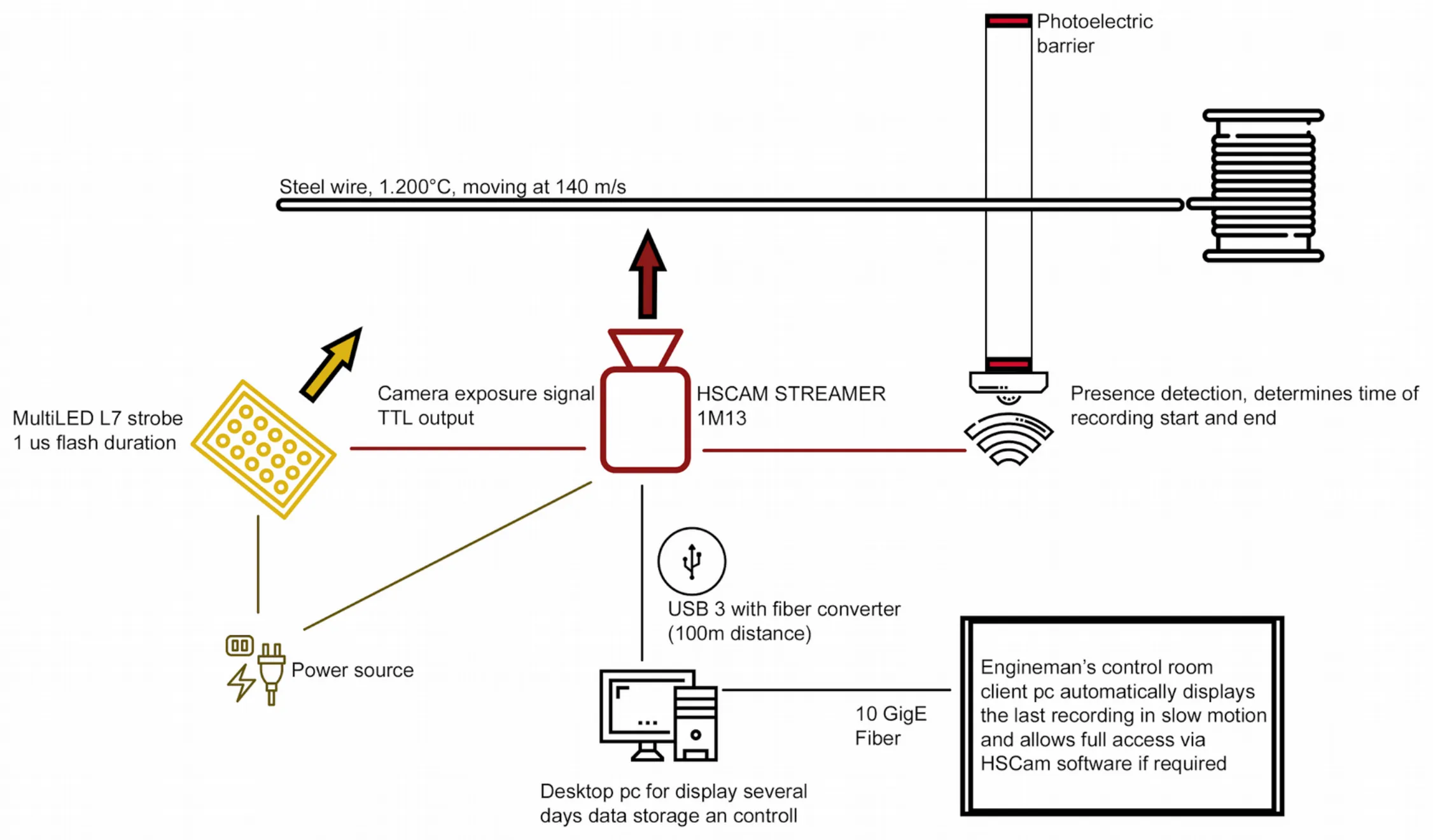
How the pieces fit together
The wire, the photoelectric barrier that times the recording, the strobe synced to the camera's exposure, and the two PCs that store and display it — from HSCAM's written Application Story.
What the mill asked for
Six requirements, agreed with the customer
1,000–3,000+ fps
At least one image every 2–10 mm of wire movement
24 / 7
Every cut and every jam recorded, with no one operating it
≥ 1 week
Of history to review when a defect is found later
Video + analogue
Measurements recorded with the images and overlaid on them
Live view
Low latency, in the engineman’s control room
Built to survive
Hundreds of °C, IR from the wire, impact from jams
Recorded footage
What the camera sees at the cut
Clips from HSCAM STREAMER recordings of wire being cut, played back slowly. The overlay in each frame is the HSCAM Viewer’s own: frame rate, resolution, data rate and compression rate.
Shear cut at 4,041 fps
- Recorded at
- 4,041 fps
- Image size
- 1,024 × 280 px
- Played at
- 15 fps · ≈270× slower
- Compression rate
- ≈ 3.5 (overlay)
The four ADC readouts in the overlay are idle in this recording; when measurement inputs are connected they show live values.
A thin strip at 10,702 fps
- Recorded at
- 10,702 fps
- Image size
- 1,024 × 104 px
- Played at
- 15 fps · ≈710× slower
- Compression rate
- ≈ 3.7 (overlay)
A smaller region of interest trades image height for frame rate: the camera reads out only the strip where the event happens.
Glowing wire at 3,000 fps
- Recorded at
- 3,000 fps
- Image size
- 1,024 × 160 px
- Played at
- 25 fps · 120× slower
- Compression rate
- ≈ 1.8 (overlay)
Each frame carries its own timestamp and frame number, which is what lets recordings be lined up with the mill’s other data.
Data volume
Why compression is part of the design
Recording every frame at full rate would bury the mill in data, and most of each image is not needed. Compressing and reducing to actual events in the camera is what lets a standard industrial PC with about six hard disks do the job.
One camera, uncompressed
~1.3 GB/s
About 5 TB per hour, 120 TB per day
One camera, one week
~840 TB
Raw, before compression and event reduction
Four cameras
~5.2 GB/s
About 4,200 TB per week, raw
Required after compression
< 1 GB/s
Across the whole production chain
Timing
A 10 ms offset puts the wire up to 1.4 m from where you think it is
Measurement systems and video systems that sync through control-system cycles can be about 10 ms apart. At 140 m/s, that means the measurement you are looking at refers to a wire position between 0 and 1.4 m away from the one in the picture, so video and measurement no longer correlate.
Temporal — timing jitter
~10 ms → nanosecond-range jitter
Without and with HSCAM’s frame-synchronous acquisition.
Spatial — synchronization accuracy
Sub-millimeter accuracy
Stated separately. It is what makes wire feed rate and slip analysable.
Survival
Built to be hit, and priced for it
Ambient temperatures can reach several hundred degrees, the wire radiates IR, and a jam can destroy equipment. Housings for camera and lights are water-cooled, protected against IR intrusion, and made of V4A steel to withstand contaminated cooling water and impact.
The glass openings are the weak point: if the wire runs into them at certain angles, the electronics inside are destroyed. It happens and cannot be avoided, so HSCAM keeps dedicated spare stock for this kind of system and offers extended warranty and service contracts with 50% off spares for destroyed parts.
Lost per 250,000 accumulated operating hours
- Housings
- 1
- Cameras
- 2
- Lights
- 4
Both camera losses are explained: one during a jam with hot wire around the housing, one by water damage after an impact. All four lights were lost to wire entering through the window.
On site
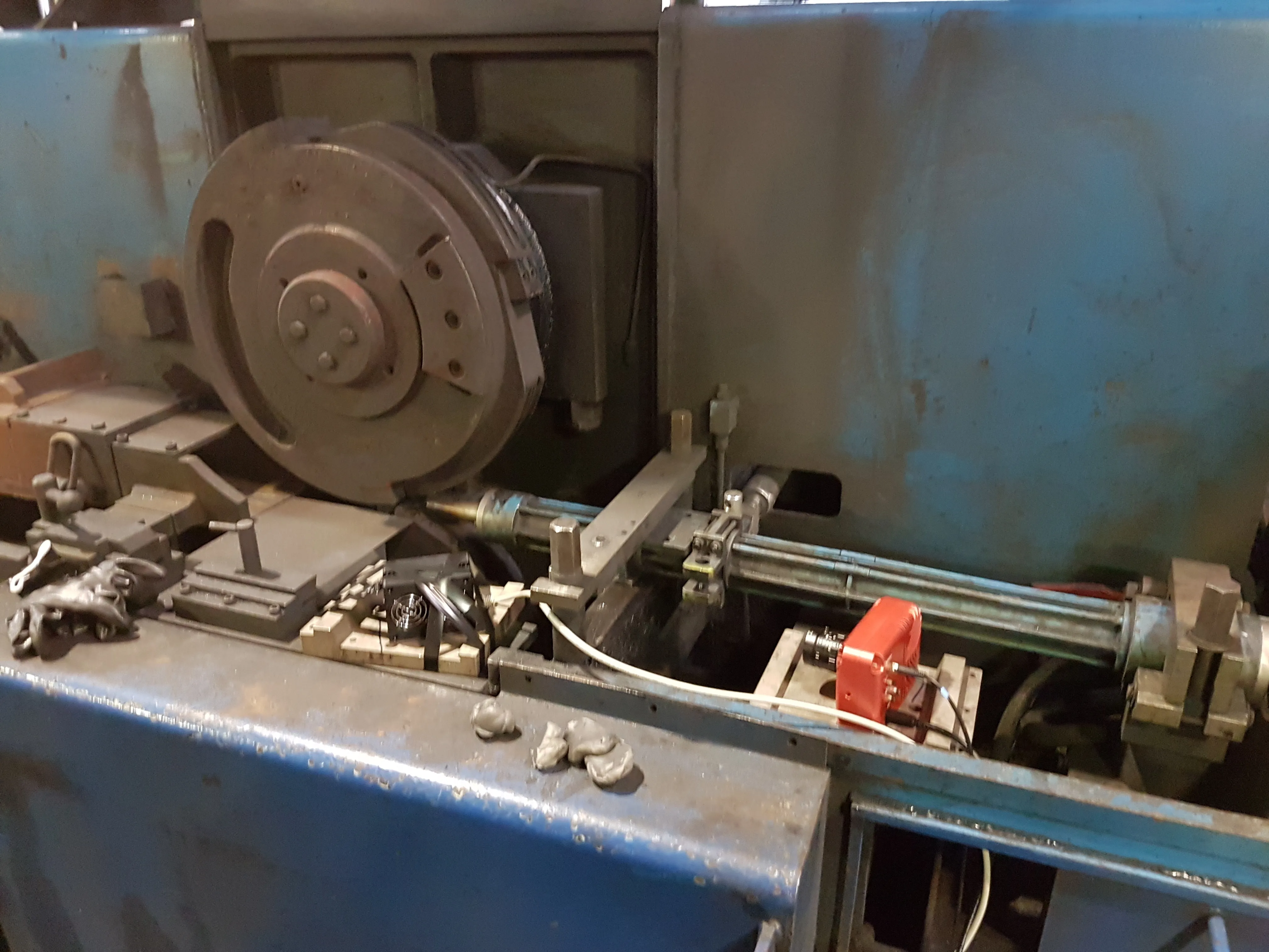
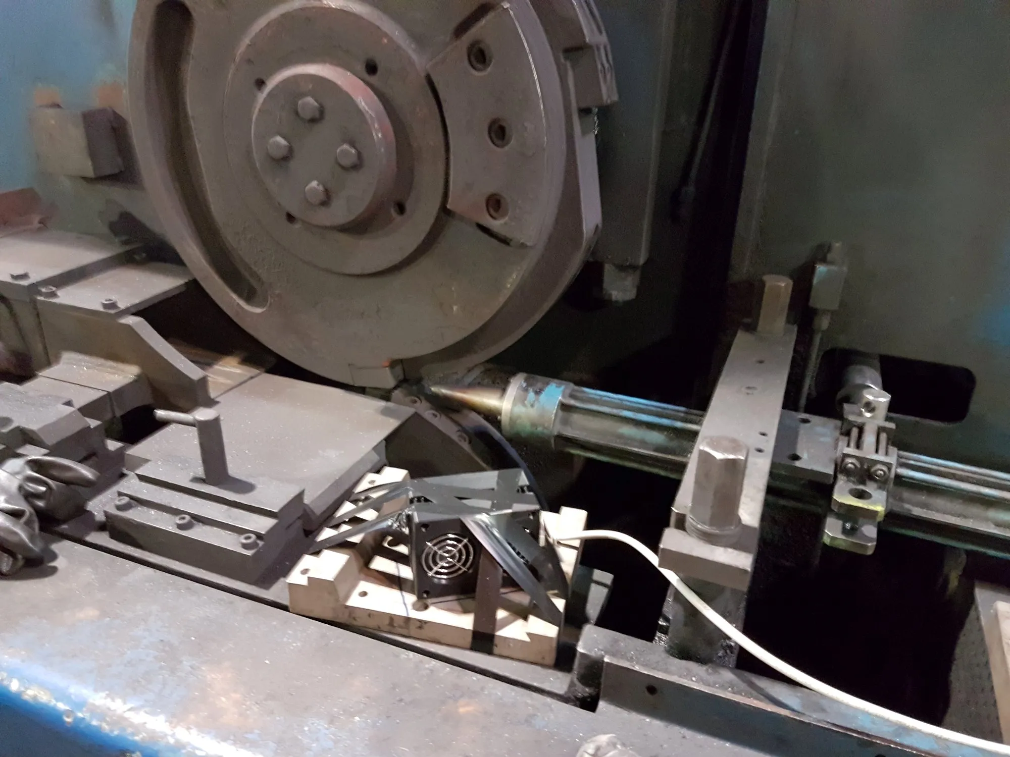
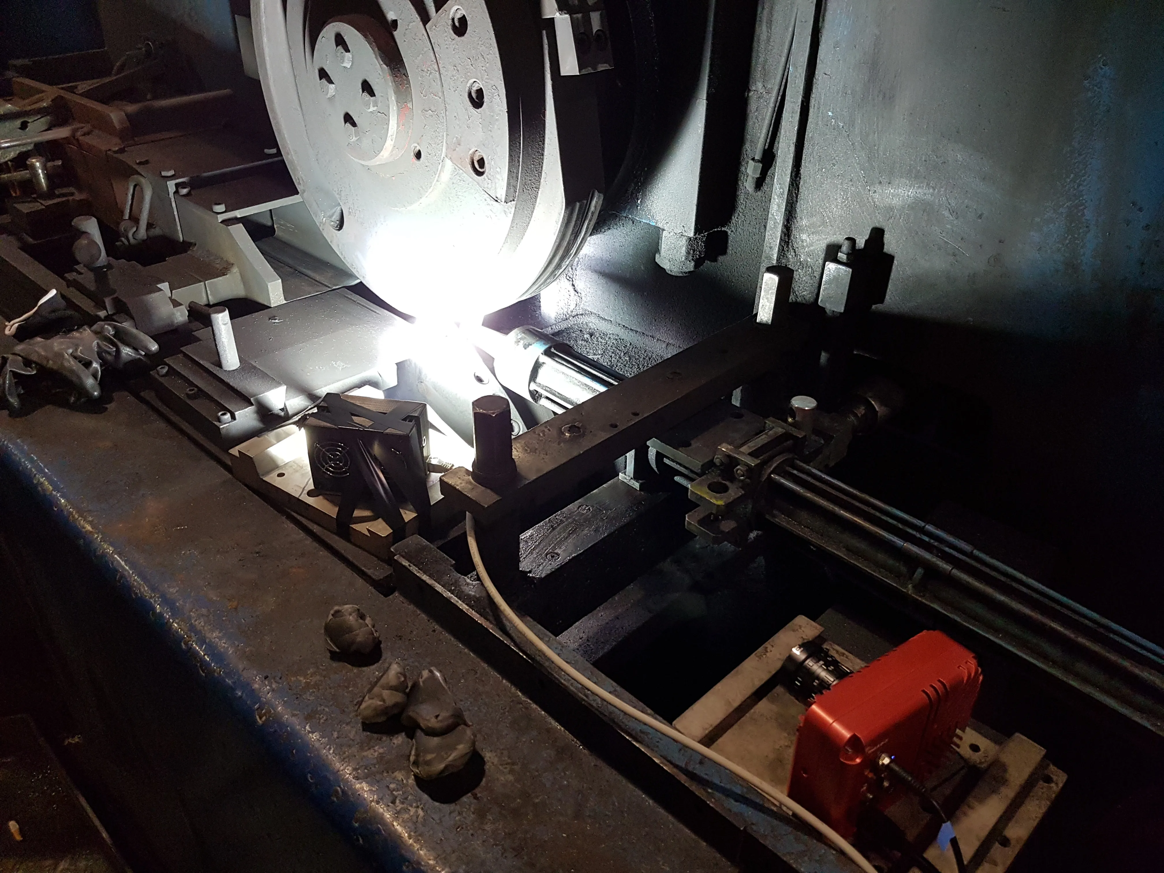
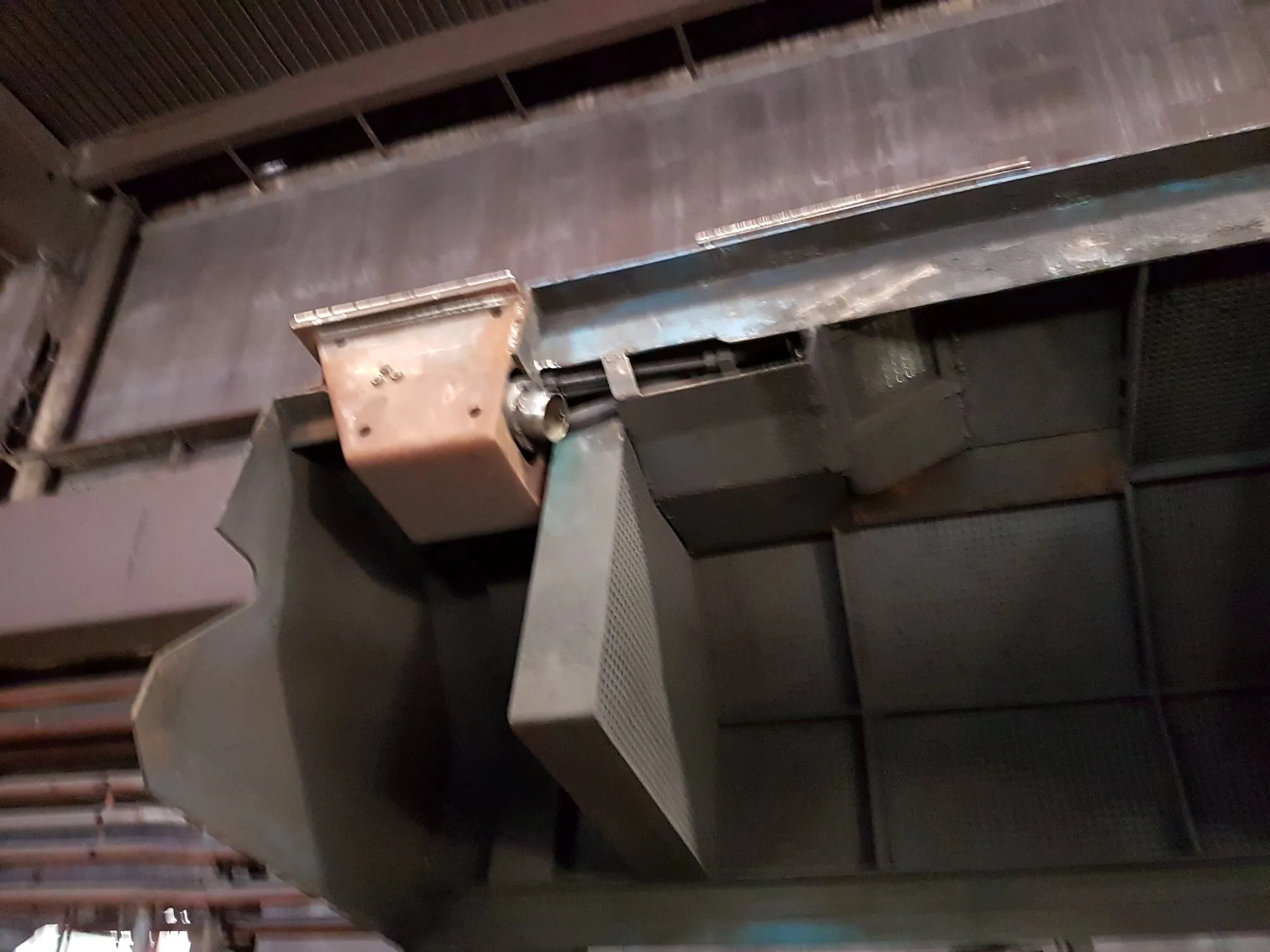
A small red camera in a very hostile place
Camera and lights sit 30–60 cm from the wire, mounted to the inside of the hood so they move into position when the hood closes.
How it works
From a photocell to a week of history
- 1
A photocell detects incoming goods
This starts the recording, with 100 ms of pre-trigger history.
- 2
Recording runs while goods are present
And stops when they leave the sensing range.
- 3
The camera compresses image data itself
Most of each frame is not needed, so the stream is reduced in the camera.
- 4
Measurements are captured on the same clock
4 internal ADC channels, extendable to 20 with the HS-DAQ.
- 5
Critical steps replay automatically
In slow motion on several displays.
- 6
Everything is kept for a week or more
So mechanical behaviour can be reviewed after a fault.
Equipment
- HSCAM STREAMER 1M13 with application-matched lens
- HSCAM Viewer, with the Viewer Scripting Plugin (Python)
- MultiLED L7 strobe light: 750,000 lumen, pulses from 100 ns
- Photocells at the start, presence and end of goods
- Fibre-optic USB3 extender, up to 150 m to the PC
- Desktop PC for display and storage (20–200 TB), client PC for the control room, 10 GigE fibre link between them
- Water-cooled V4A steel housings for camera and lights
Customization
Four small Python scripts do the mill’s bidding
Camera settings, analogue channels, recording behaviour and image processing are all controllable from the HSCAM Viewer Scripting Plugin.
Photocell trigger
The camera captures the photocell and generates the trigger event; recording starts with 100 ms pre-trigger. Image processing can drive the trigger instead.
Automatic file handling
A template-based Viewer configuration creates the files and distributes them over the network.
Housekeeping
A second script deletes the oldest recordings so there is always space for new ones.
Plant integration
For some customers HSCAM has written scripts that follow the recording behaviour to data from the production system.
Outcome
What the installation delivers
Figures from this one deployment.
- Continuous 24/7 streaming over USB3 at more than 1,300 fps, thanks to edge-keeping compression in the camera.
- Live view and trigger options let the process be monitored in real time, not only reviewed afterwards.
- Less data to move makes the transport layer more robust, and a week or more of production history fits on a standard PC.
- Image-synchronous measurements make the process analysable, not just viewable.
- Scripting makes it easy to adapt the process behaviour to the mill.
- Fibre-optic USB3 extension keeps the computers away from the heat and impact.
Equipment
The camera behind it
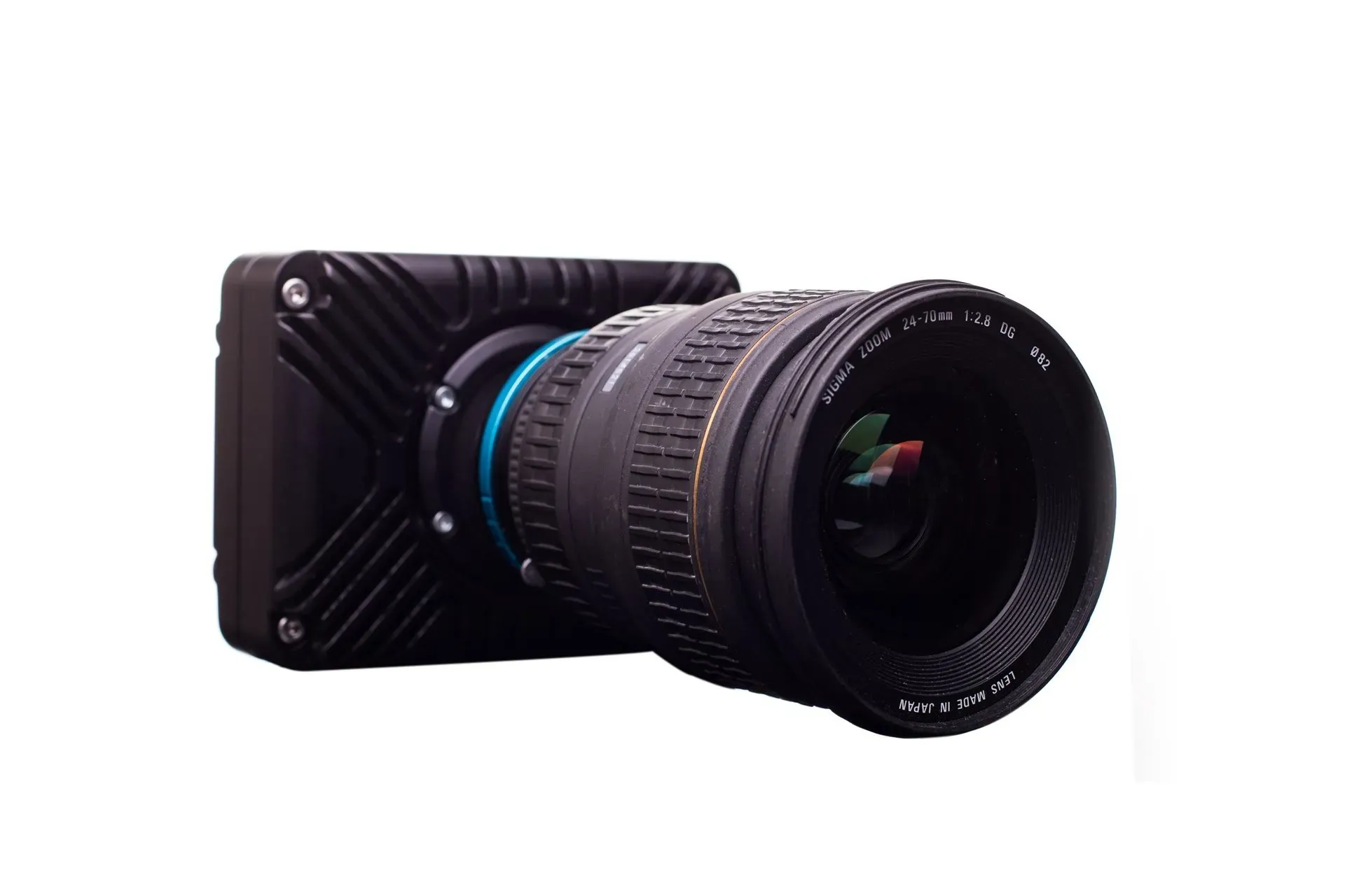
HSCAM STREAMER 1M13
The camera installed at the shear, running this deployment.
View product →Related
Same principle, other setups
Recognize this on your own line?
I have a similar problem →Talk to an engineer about your production line
Tell us your material speed, environment and how long you need to keep the recordings.
HSCAM GmbH · Angerstraße 40–42, Haus B · 04177 Leipzig, Germanycontact@hscam.com · www.hscam.com